1. Login

Following the installation of the CADLIVE Simulator, open http://kurata01.bse.kyutech.ac.jp/TEST/Life/index.html on a PC browser to display the screen shown in Fig. 1-1. Input the user name, subsequently his/her password to start up simulation.

If there is anything wrong with calculation and you want to kill your job, access the site of http://kurata01.bse.kyutech.ac.jp/TEST/Life/kill, and push the kill simulator button.

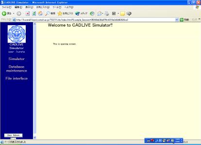
Fig. 1-1 Startup screen

2. User registration

Click the [User Admin] button under the left side of the screen to display the screen shown in Fig. 2-1. This operation is restricted to the persons who are registered as administrators. Registration is carried out by inputting the user name, his/her password, and admin/user.

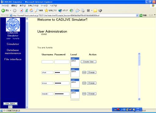
Fig. 2-1Screen for registering users

The persons who have the admin account are able to delete any accounts and their data, but ones with the user account are not able to access the other accounts.

3. DB maintenance

Click the [Database Maintenance] button, the screen transits as shown in Fig. 3-1

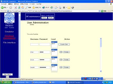
Fig. 3-1 Database maintenance

Clicking the [Delete] button displays the lists of registered data (Users: their own data, Admin: the data of all the accounts), as shown in Fig.3-2. Users are able to delete the data by clicking the corresponding checkbox and by clicking the [Delete] button. Users save their data at their convenient time during the process of simulation.

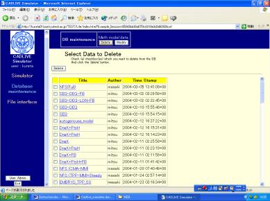
Fig. 3-2 Mathematical model data

Clicking the [Modify] button displays the list of the registered data as shown in Fig. 3-3, which is similar to that as shown in Fig.3-2.

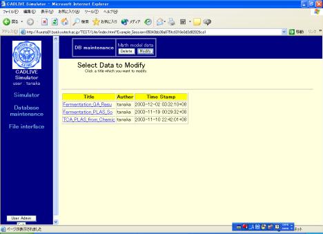
Fig. 3-3 Selection for mathematical model data

Clicking the data title that users want to modify displays the new screen shown in Fig. 3-4, where they edit their models. Clicking the [Save to DB] button registers the modified data on the database. Notice that users have to learn the instruction of the simulator to edit their data manually.

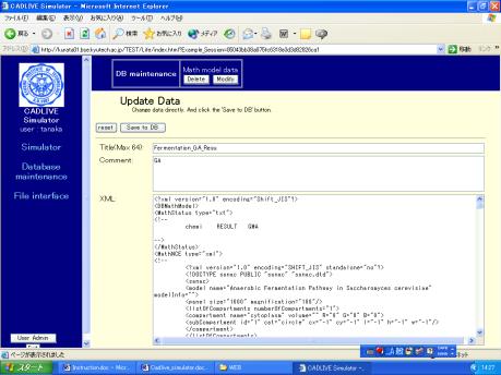
Fig. 3-4 Editing mathematical model data

4. File interface

Clicking the [File Interface] button changes the upper region of the screen as shown in Fig. 4-1, where users change their data between the database and their PC.

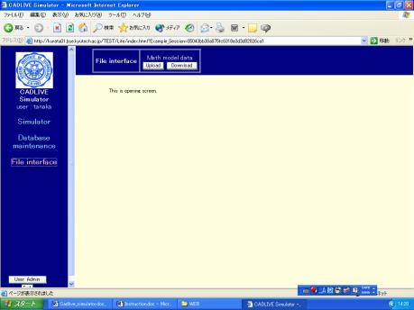
Fig. 4-1File interface

Clicking the [Upload] button displays the screen (Fig. 4-2), where users are able to register their data.

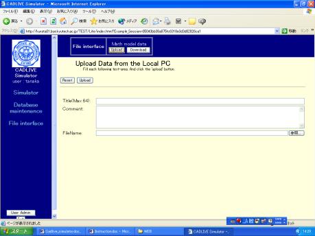
Fig. 4-2 Upload data from a local PC

On the other hand, clicking the [Download] button displays the list of the registered data, where users see the content by clicking the data title and download it to their PC.

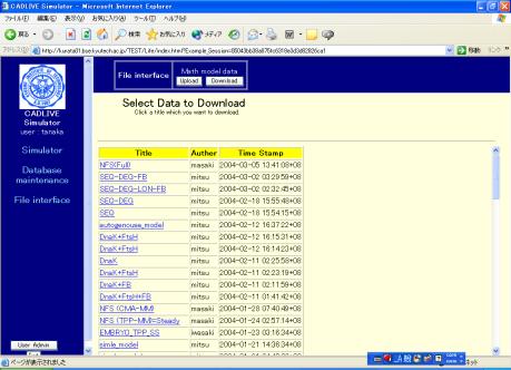
Fig. 4-3 Select data to download

5. Simulator

5.1 Start screen

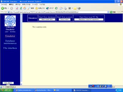
Clicking the "Simulator" button changes the upper region of the screen as shown in Fig.5-1.

Fig. 5-1Startup for simulator

5.2 Upload of data for regulator-reaction equations

On the startup screen (Fig. 5-1), clicking the [Regulator-reaction equations] button displays the screen (Fig. 5-2), where users select the data file for regulator-reaction equations from their PC. Users are required to click the buttons within the white screen, not to carelessly click the buttons of the browser.

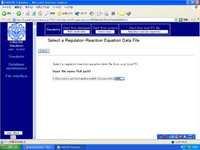
Fig. 5-2 Select of regulator-reaction equation data file

5.3 Selection of conversion methods

Selecting an appropriate data file displays the screen (Fig. 5-3), where users choose the conversion methods with respect to gene-protein layer and metabolic layer, respectively.

The conversion method can be selected out of the following methods:

Gene-Protein layer:

- CMA

- TPP_STEADYSTATE_1

- TPP_STEADYSTATE_2

- TPP_RAPID

Metabolic layer:

- GMA

- MM

- SAME_AS_GENE-PROTEIN

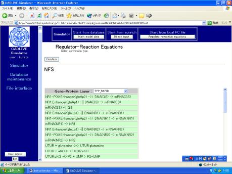
Fig. 5-3 Selection of conversion methods

Following the selection of the conversion methods, clicking the [Confirm] button displays the confirmation screen that is similar to Fig. 5-3.

5.4 Editing mathematical model

Clicking the [Submit] button on the confirmation screen (Fig. 5-3) parses the regulator-reaction equations, converting them into the mathematical model according to the selected conversion method. The resultant mathematical model is displayed on the screen (Fig. 5-4).

Fig. 5-4 Mathematical models

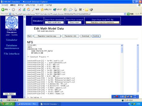
This screen mainly has seven parts: the header, the definition of constant players, the definition of variables, the definition of the employed parameter labels, the definition of kinetic parameters, the definition of intermediate mathematical expressions, the definition of algebraic equations, and the definition of differential equations.

Clicking the [Regulator-reaction eqs.] button displays another window for showing regulator-reaction equations. Clicking the [Parameter info.] button shows the parameter information. The [Download] button enables users to download various data files to their local PC. Clicking the [Confirm] button displays the confirmation screen. If there is no problem, click the [Submit] button. The detailed instruction is referred in the documents regarding checkdae.

5.5 Selecting analysis types

Clicking the [Submit] button on the confirmation screen displays the screen (Fig. 5-5), where users select the analytical type for a mathematical model.

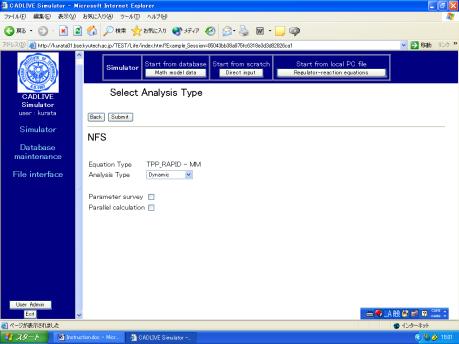
Fig. 5-5 Selection of analytical types

As "Analsys type", users can choose either “Dynamic” or “Steady-state”. “ Dynamic” simulates the time evolution of the concentrations by calculating differential and algebraic equations, and “Steady-state” calculates the concentrations at steady state by solving algebraic equations. The checkbox of "Parameter survey" determines if the simulator surveys the parameter space. Checking the checkbox of "Parallel calculation" carries out parallel calculation that employs the Message Passing Interface (MPI). Notice that the checkbox of "Parallel calculation" cannot be selected prior to checking the parameter survey.

The checkbox of "Use S-system", which employs S-system differential equations, appears only under the condition that the steady-state concentrations have been solved.

5.6 Input for control data

Clicking the [Submit] button on the selection screen for analytical types displays the screen for input of the control data (Fig. 5-6). Following data input, clicking the [Confirm] button shows the confirmation screen. The detailed explanation is described elsewhere.

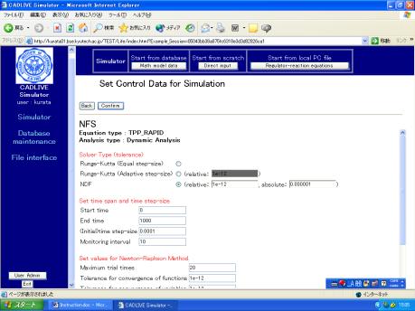
Fig. 5-6 Set control data for simulation

5.7 Input of parameters

Clicking the [Submit] button on the confirmation screen for setting control data for simulation displays the new screen (Fig. 5-7-1), where users input the values for the kinetic parameters and initial values. The detailed explanation is described elsewhere.

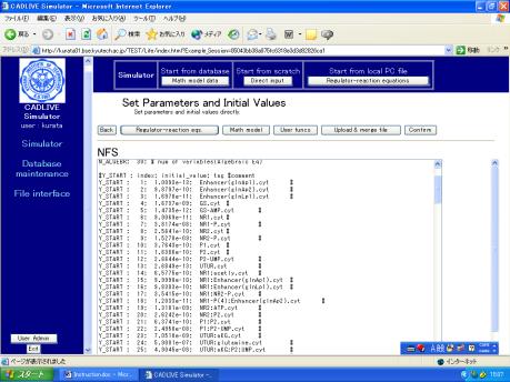
Fig. 5-7-1 Setting parameters and initial values

The [Initial val.] button, which does not appear on the screen until the “Save for input” button is carried out by the previous simulation, displays the final values of the time course data that have been simulated. Those values are copied and pasted as the initial values on the file for setting parameter and initial values. The initial values is required for solving the steady state concentrations of the algebraic equations

Clicking the [Upload & merge File] displays the screen (Fig. 5-7-2). After clicking the [Confirmation] button, clicking the [Submit] button transit to the confirmation screen.

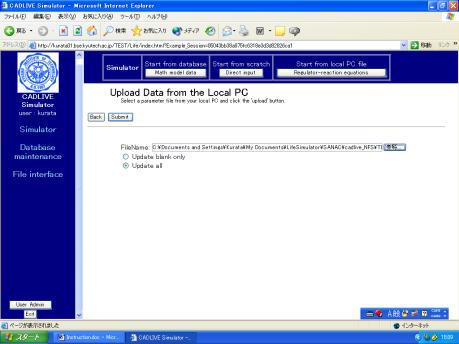
Fig. 5-7-2 Uploading data from a local PC

The parameter file that has been made according to the rules of the simulator is input in the box of "FileName". Clicking the [Upload] button displays the previous screen (Fig. 5-7-1), where the parameters are automatically input from the uploaded file. Checking the box of "Upload blank only" does not update the existing parameters and initial values. Checking the box of "Upload all" replaces all the data by those of the uploaded parameter file.

5.8 Result indication

Clicking the [Submit] button on the confirmation screen starts simulation and displays the results (Fig. 5-8).

Fig. 5-8 Results

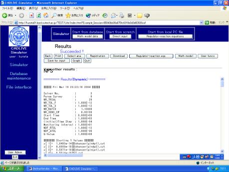
When the simulation is successfully completed, the results are shown on the screen, which contains the log including the calculation time. The final runs of time evolution and steady-state analysis are saved as the results, respectively. When simulation fails, the log is shown first, subsequently displaying the input file.

The button of [Save for input] stores the concentrations at the final time or the steady state concentrations, which can be used for the subsequent analysis of the time-evolution dynamics and the steady state analysis, respectively. Notice the [Initial val.] button (Fig. 5-7-1).

Clicking the [Graph] button, which appears when the time-evolution of "dynamic" is simulated successfully, opens the window that indicates the results.

5.9 Database registration

The screen for indicating the results (Fig. 5-8) has the [Registration] button. Clicking the [Registration] button shows the final confirmation screen that has also the button of [Registration]. Clicking it displays the screen for "Insert New Data from the Simulator" (Fig. 5-9). Following inputting the title and comments, clicking the [Save to DB] button saves a series of simulation data as a mathematical model in the database.

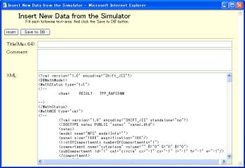
Fig. 5-9 Registration of data in database

5.10 Data download

The screen for results (Fig. 5-8) also has the [Download] button. Clicking it displays the download screen (Fig. 5-10)

Fig. 5-10 Download

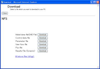
The data files that have been built are listed. The clicked files are downloaded to a local PC.

5.11 Selecting a mathematical model

Clicking the [Math model data] button on the "Start" screen (Fig. 5-1) displays the screen for "Select Data to Simulate" (Fig. 5-11-1).

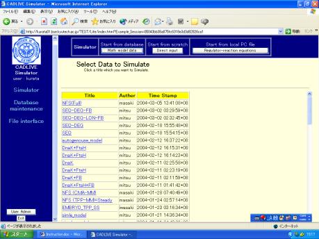
Fig. 5-11-1 Selection of a mathematical model

Clicking the title displays the content of the data, as shown in Fig. 5-11-2.

Fig. 5-11-2 Confirmation of a mathematical model

5.12 Selecting job (Mathematical model)

Clicking the [Go Simulator] button on the "Confirmation Data for Simulation" displays the new screen (Fig. 5-12)

Fig. 5-12 Selection of a job

Fig. 5-12 shows three choices, when a mathematical model has been registered after the simulation was completed. If simulation has not been completed, this screen indicates only the above two choices.

Go to [Edit User Functions]. :jump DAE editing screen (Fig. 5-4)

Go to [Select Analysis Type]. :jump Calculation method selection screen (Fig.5-5).

Go to [Results]. :jump the result screen (Fig.5-8).

5.13 Direct edition of mathematical equations

On the "Start" screen (Fig. 5-1), clicking the [Direct input] button displays the screen (Fig. 5-13). Following the input of a title and comment, clicking the [Submit] button displays the screen for indicating mathematical equations (Fig. 5-1), where the identification lines exist, but no data is contained. Users can make mathematical equations according to the rules of the simulator, which is described elsewhere (Commentary for PARSEDAE).

Fig. 5-13 Direct input of a mathematical model

6. Graph visualization

6.1 Setting graph data

Clicking the [Graph] button displays the window of "Set Graph Data".

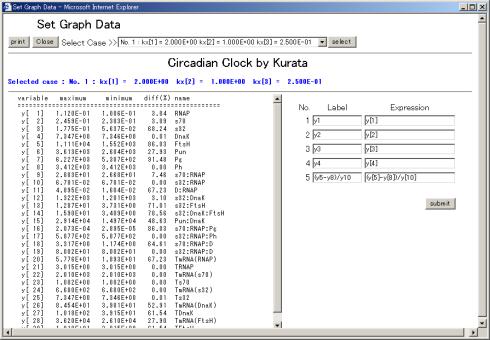
Fig. 6-1 Setting graph data

Fig. 6-1 shows the results of the parameter surveys, where the pulldown menu is used for selecting a case of the simulation. Selecting a case from this pulldown menu, clicking the [Select] button turns the blue characters to the values for the selected case.

The right hand side of the screen defines the definition of data that will be plotted on a graph, and can indicate five series of labels and expressions. As default, y1 – y5 and y[1] – y[5] are set as labels and expressions, respectively. Empty labels and expressions are not allowed. The variables y[i], calculation symbols +, -, X, /, parentheses (,), and time T are allowed to be used for describing the mathematical expression. After setting them, click the [Submit] button.

6.2 Set for graph display

Clicking the [Submit] button on the screen for setting graph data (Fig. 6-1) displays the screen (Fig. 6-2), where the scaling factor and the regions of the X-axis and Y-axis are automatically calculated based on the expression and the minimum/maximum values to visualize the five time-evolution well. The left hand side of the lower screen shows the maximum and minimum values, and the changing ratio provided by:

(Maximum - Minimum) / Max (|Maximum|, |Minimum|) X 100.

Users are able to change the labels, the scaling factors, and the color of the lines.

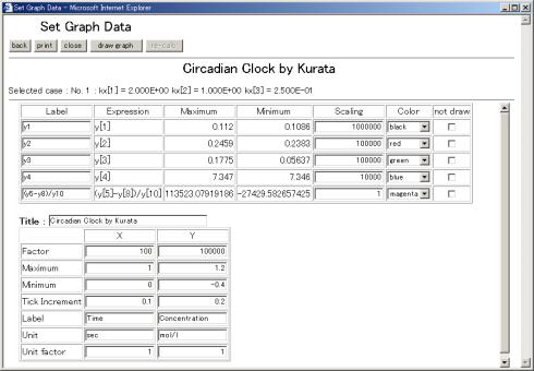
Fig. 6-2 Setting graph data

Checking the checkbox of “not draw” omits its time evolution from the graph. Clicking some checkboxes of “not draw” disables the [Draw graph] button, instead enables the [Rre-calc] button to work. The button [Re-calc] recalculates the scaling factors and the regions for the X/Y-axises. The table on the lower screen is set for the X/Y-axises. X indicates time, and Y the concentrations of variables.

In the above example, the label of the X-axis is Time [x 100 sec], where the numerical label is from 0 to 1.0 at the interval of 0.1. If users want to change the label: the numerical label is from 0 to 100 at the interval of 10, they set the scaling factor, the maximum and the tick increment as 1, 100, and 10, respectively. The X label becomes Time [sec]. The unit factor is the scaling factor for unit. For example, the [msec] label is changed to the [sec] label by multiplying 0.001 as the scaling factor.

6.3 Graph display

Clicking the [Draw graph] button on the screen for setting a graph (Fig. 6-3) displays the results of time-evolution data.

Fig. 6-3 Graph display

The [no legend] button omits the legends. The [Set details] button is able to change the color of the graph and other graph expressions.

6.4 Details of graph

Clicking the [Set details] button displays the window (Fig.6-4). Users can change the style of the graph by inputting the value in the boxes. The values of the graph size and the location of the legends are determined by using pixel units. The location of the legend is determined by the coordinate of the left and upper legend

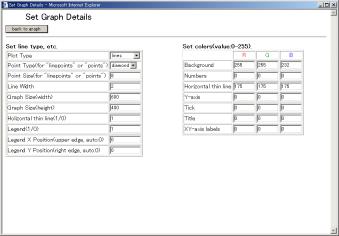
Fig. 6-4 Detailed setting for a graph