1.
Objectives
Sensitivity analysis shows how a biochemical system responds to perturbations or uncertainties. Among many methods for system analysis, the sensitivity and stability analysis is useful for characterizing the robustness of the mathematical at a steady-state level, and allows one to determine which parameters have the most effect on the model, or which factors cause to the system to oscillate. S-system is employed to analyze the various sensitivities and stability of the system at its steady state, because the use of S-system solves them in symbolic form. In this module, ordinary differential equations such as TT, CMA, GMA, and MM are converted into S-system to analyze the sensitivities and stability.
TT: ordinary transcription and translation equations
CMA : conventional mass action
GMA: general mass action
MM : simplified Michaelis-Menten equations
2.
Introduction of S-system
We show how S-system is derived from ordinary differential equations, and how the stability and sensitivity are defined at the steady state.
2.1 S-system conversion
Ordinary
differential equations are divided into the positive terms and negative terms:
![]() , (i
= 1,....,n,....n+m)
(1),
, (i
= 1,....,n,....n+m)
(1),
where ![]() is the sum of positive terms, and
is the sum of positive terms, and ![]() is the sum of
negative terms. Generally, S-system is given by:
is the sum of
negative terms. Generally, S-system is given by:
![]() (2),
(2),
where X1,…, Xn
are the dependent variables, whose values vary with time, and Xn+1,…,Xn+m
are the independent variables, whose values are fixed as constants. When the
concentrations of the dependent variables are given at the steady state, the
coefficients (gij, hij, ai, bi) of
S-system are solved from Eqs. (1, 2) in symbolic form:
 (3)
(3)
 (4)
(4)
where gij and hij are the kinetic order and ai and bi are the rate constants. At the
steady state:
![]() ,
,
we can take logarithms on both sides of Eq. (2), the equation reduces to a linear equation:
![]() ,
,
or
![]() (5).
(5).
Substituting ![]() . The equations (5) is changed to the vector-matrix
expression:
. The equations (5) is changed to the vector-matrix
expression:
![]() (6).
(6).
We substitute the matrixes as follows,
![]()
to obtain the equation:
![]() (7)
(7)
where AD is the
coefficient matrix of the kinetic order regarding dependent variables, AI
is the coefficient matrix of the kinetic order regarding independent variables,
![]() is the solution
vector of dependent variables,
is the solution
vector of dependent variables, ![]() is the vector of
independent variables, and
is the vector of
independent variables, and ![]() is the vector
regarding the rate constants. Consequently, the vector of the dependent
variables is symbolically solved as:
is the vector
regarding the rate constants. Consequently, the vector of the dependent
variables is symbolically solved as:
![]() (8).
(8).
2.2 Sensitivity analysis
We define five types of gains and sensitivities. The detailed derivation of them are described elsewhere. Here, we explain the mathematical definition of them.
2.2.1. Logarithmic Gain of a metabolite
In order to answer the question of how a
relative change in an independent variable affect the steady-state
concentration of a metabolite, the logarithmic gains of a metabolite ![]() is defined in
terms of the coefficient matrixes
is defined in
terms of the coefficient matrixes ![]() and
and ![]() as:
as:
![]() (9).
(9).
2.2.2. Logarithmic gain of a flux
In order to answer the question of how a
relative change in a flux affect the steady-state concentration of a
metabolite, the logarithmic gains of a flux ![]() is defined in
terms of the coefficient matrices
is defined in
terms of the coefficient matrices ![]() and
and ![]() as:
as:
![]() (10).
(10).
2.2.3. Sensitivity with respect to a rate constant
In order to answer the question of how a relative change in a rate constant affect the steady state concentration of a metabolite, we solve the sensitivity with respect to rate constants, which is defined as:
![]() (11),
(11),
and
![]() (12).
(12).
These sensitivities are expressed using vectors and matrixes as
![]() (13),
(13),
![]() (14).
(14).
2.2.4. Sensitivity of dependent variables with respect to a kinetic order
In order to answer the question of how a relative change in a kinetic order affect the steady-state concentration of a metabolite, we define the sensitivity with respect to the kinetic order as follows,
![]() (15),
(15),
![]() (16).
(16).
The partial derivatives of Eq. (8) regarding gij are provided by:
![]() , (17)
, (17)
or
![]() . (18)
. (18)
Therefore,
![]() (19)
(19)
![]() (20).
(20).
2.2.5. Sensitivity of a flux to a rate constant
In order to answer the question of how a relative change in a rate constant affect the steady-state concentration of a flux, we define the sensitivity with respect to a rate constant.
We take logarithms in the first term of the right hand side of S-system:
![]() (21)
(21)
![]() (22)
(22)
In analogy, partial derivatives of Eq.(21) with respect to lnβi gives:
![]() (23).
(23).
2.2.6. Sensitivity of a flux with respect to a kinetic order
In order to answer the question of how a relative change in a kinetic order affect the steady-state concentration of a flux, we define the sensitivity with respect to a kinetic order.
The partial derivatives of Eq. (21) with respect of ln gij is provided as:
![]() (24).
(24).
In analogy, the partial derivatives of Eq. (21) with respect of ln hij is provided as:
![]() (25).
(25).
2.3 Stability analysis
Defining the equation:
δXk = Xk − XkS (XkS steady state),
we apply the first order approximation to Eq. (2) to obtain:
 (26),
(26),
or
![]() (27),
(27),
As ![]() , we define:
, we define:
to deduce to:
![]() (28).
(28).
Stability at the steady state is investigated by solving the eigenvalues of the coefficient matrix consisting of:
![]() .
.
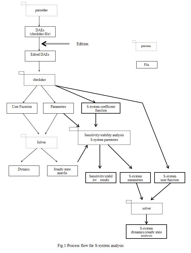
3
Process flow
Fig. 1 shows the whole processes of the simulator, where the process flow of S-system mainly consists of three parts:
1) creation of the S-system coefficient file, which consists of the kinetic orders and rate constants that are solved in symbolic form at the steady state,
2) creation of the S-system parameter file (the coefficients and steady-state concentrations) necessary for sensitivity/stability analysis, which is made using the S-system coefficient function and the steady state concentrations.
3) simulation of S-system.
The checkdae module carries out the process of 1), following that the user function for ordinary differential equations (TT, CMA, GMA, MM) have been established. However, the checkdae module does not convert the differential and algebraic equations (DAEs), because they cannot be converted into S-system directly. The program module carries out the analysis of the sensitivities and stability of S-system by linking the S-system coefficient function to the steady-state concentrations. The concentrations at the steady state must be solved before this analysis.