1. Login
Following
the installation of the CADLIVE Simulator, open http://kurata01.bse.kyutech.ac.jp/TEST/Life/index.html on a PC browser to display the screen(Fig. 1-1). Input the user name,
subsequently his/her password to start up simulation.
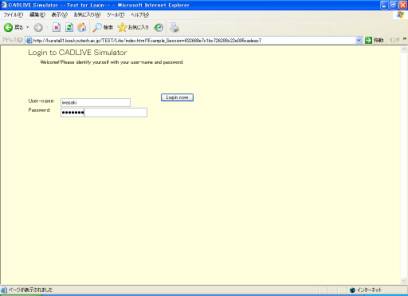
Fig. 1-1 Login
screen
2. Startup simulator
Clicking the "Simulator" button on the left hand side (Fig. 2-1) changes the upper region of the screen, as shown in Fig.2-2
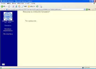
Fig. 2-1Startup menu
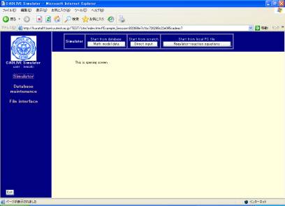
3. Upload of data for regulator-reaction equations
Clicking the [Regulator-reaction equations] button (Fig. 2-2) displays the new screen. Select the XML data file for the regulator-reaction equations (HSR_demo.xml) from users’ PC (Fig. 3-1). The data file should be described by using the CADLIVE Editors. Users are required to click the buttons within the screen of CADLIVE, not to carelessly click those of the browser.
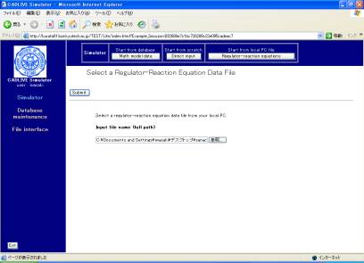
Fig.
3-1 Upload of a regulator-reaction equation file from a PC
4. Selection of conversion methods
The table that indicates the selected regulator-reaction equations appears on the screen (Fig. 4-1). Users choose the conversion method with respect to gene-protein layer, because the heat shock response does not contain the metabolic layer. Select TPP_RAPID.
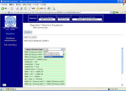
Fig. 4-1
Selection of conversion methods
Following
the selection of the conversion method, clicking the [Confirm] button displays
the confirmation screen (Fig. 4-2) that is similar to Fig. 4-1.
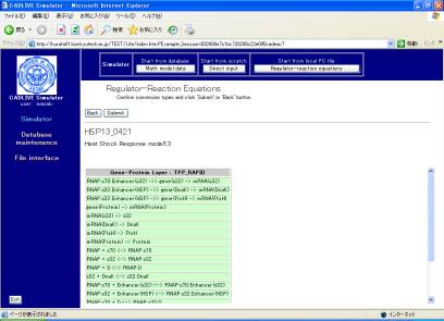
Fig. 4-2
Confirmation screen for the regulator-reaction equations
5. Editing Mathematical Model (DAEs)
Clicking the [Submit] button on the confirmation screen (Fig. 4-2) parses the regulator-reaction equations, converting them into the mathematical model according to the selected conversion method. The resultant mathematical model is displayed as shown in Fig. 5-1.
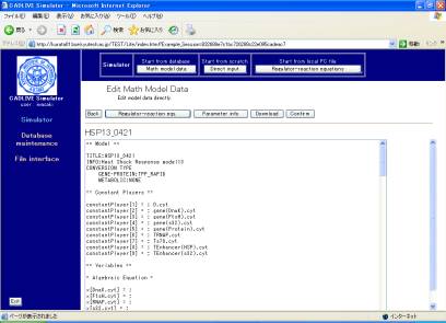
Fig. 5-1 Mathematical model that is obtained from regulator-reaction equations
This screen mainly has seven parts: the header, the definition of constant players, the definition of variables, the definition of the employed parameter labels, the definition of kinetic parameters, the definition of intermediate mathematical expressions, the definition of algebraic equations, and the definition of differential equations.
Clicking the [Regulator-reaction eqs.] button displays another window that shows regulator-reaction equations. Clicking the [Parameter info.] button shows the parameter information. The [Download] button enables users to download various data files to their local PC.
Clicking the [Confirm] button displays the confirmation screen (Fig. 5-2) that is similar to Fig. 5-1. If there is no problem, click the [Submit] button.
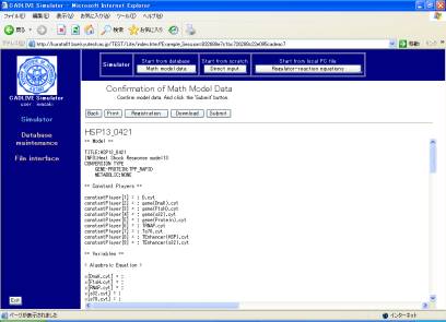
Fig. 5-2 Confirmation screen for a mathematical model
6. Selecting analysis types
Clicking the [Submit] button on the confirmation screen displays the screen (Fig. 6-1), where users select the method for numerical simulation. Select “Dynamic” as analysis type.
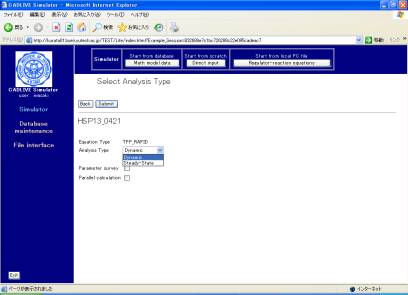
Fig. 6-1Selection of analysis type
As "Analsys type", users can choose either “Dynamic” or “Steady-state”. “ Dynamic” simulates the time evolution of the concentrations by calculating DAEs, and “Steady-state” calculates the concentrations at steady state by solving algebraic equations. The checkbox of "Parameter survey" determines if the simulator surveys the parameter space. Checking the checkbox of "Parallel calculation" carries out parallel calculation that employs the Message Passing Interface (MPI). Notice that the checkbox of "Parallel calculation" cannot be selected prior to checking the parameter survey.
7 Input for control data
Clicking
the [Submit] button on the screen for selecting analytical type displays the
screen for input of the control data (Fig. 7-1). Here, input the data, as
provided by the following table
|
Solver Type
(tolerance) |
|
|
Runge-Kutta (Adaptive step-size) |
relative: 1e-12 absolute 0.000001 |
|
Set time span and
time step-size. |
|
|
Start time |
0 |
|
End time |
100 |
|
(Initial)time step-size |
0.0001 |
|
Monitoring interval |
1 |
|
Set values for
Newton-Raphson Method. |
|
|
Maximum trial times |
20 |
|
Tolerance for convergence of functions |
1e-12 |
|
Tolerance for convergence of variables |
1e-12 |
|
Ratio of changing parameters |
1.1 |
|
Other |
|
|
G-value |
1.0 |
|
Y default value |
0.01 |
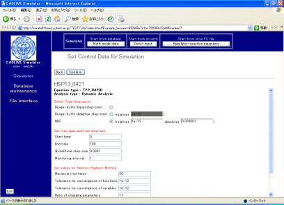
Fig. 7-1 Set control data for simulation
Following data input, clicking the [Confirm] button shows the confirmation screen (Fig. 7-2).
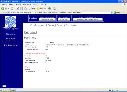
Fig. 7-2 Confirmation screen
8. Input of parameters
Following
confirming the control data for simulation, clicking the [Submit] button on the
screen (Fig. 7-2) displays the new screen (Fig. 8-1), where users input the
kinetic parameters and initial values.
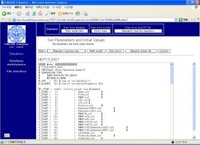
Fig. 8-1 Setting parameters and initial values
In this example, we presented the parameters and initial values that well simulated the heat shock response. Click the [Upload & merge File] button to display the screen (Fig. 8-2).
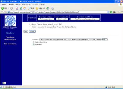
Fig. 8-2 Uploading a parameter file from the local PC
The parameter file that has been made (TPP_Param_HSR.txt) should be input in the box of "FileName". Check the box of "Update all" and click the [Submit] button. The parameters and initial values are automatically input into the mathematical model, as shown in Fig. 8-3

Fig. 8-3 Uploaded parameters and initial values
Users are allowed to edit the mathematical model on the screen (Fig. 8-3) directly. We ask users to learn “Time event”, which causes the certain parameters to change. In the heat shock response, the temperature changes abruptly at 50 min, accompanied by the altered values of the parameters: kx[4] and kp[1]. Set the time event, as shown in Fig. 8-4
#T_EVENT ; name;
index; time; value; #comment
T_EVENT ; kx; 2; 60;
150; #comment
T_EVENT ; kp; 1; 60;
80; #comment
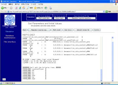
Fig. 8-4 Set of time event
Following clicking the [Confirm] button, clicking the [Submit] button (Fig. 8-5) starts calculation.
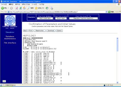
Fig. 8-5 Startup calculation
9. Result indication
The resultant time course data are displayed (Fig. 9-1), which contain the log regarding the calculation time. When simulation fails, the log is shown first, subsequently displaying the input file.
The button of [Save for input] stores the resultant data as the initial values for the subsequent simulation (Fig. 9-1), which is obtained by the [Initial val.] button. The concentrations at the final time and the steady state concentrations can be saved for the subsequent analysis of the time-evolution dynamics and the steady state, respectively. This [Initial val.] button will be not displayed when parameter survey has been carried out.
Clicking the [Graph] button, which is displayed when the time-evolution (Dynamic) is successfully simulated, opens the window for visualizing the results.
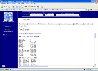
Fig. 9-1 Results
The screens for indicating the results (Fig. 9-1) have the [Registration] button. Clicking the [Registration] button shows the “Registration to the DB” screen (Fig. 9-2) that has also the button of [Registration]. Clicking it saves a series of simulation data as a mathematical model in the database.
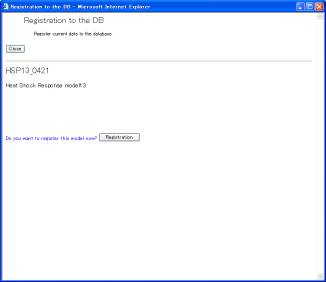
Fig. 9-2 Registration of Data in Database
The screen for results (Fig. 9-2) has the [Download] button. Clicking it displays the download screen (Fig. 9-3). The clicked files are downloaded to a local PC.
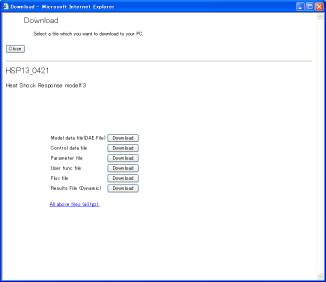
Fig. 9-3
Download
10. Graph visualization
In the screen (Fig. 9-1), clicking the [Graph] button displays the window of "Set Graph Data" (Fig. 10-1).
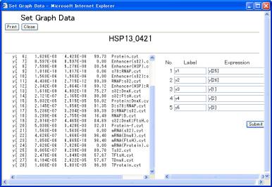
Fig. 10-1.Setting graph data
The right hand side of the screen defines the definition of data that will be plotted on a graph, and can indicate five series of labels and expressions. As default, y1 – y5 and y[1] – y[5] are set as labels and expressions, respectively. Empty labels and expressions are not allowed. The variables y[i], calculation symbols +, -, X, /, parentheses (,), and time T are allowed to be used for describing the mathematical expression. Here, set y[25], y[26], y[1], y[2], and y[3]. After setting them, clicking the [Submit] button displays the screen (Fig. 10-2), where the scaling factor and the regions of X-axis and Y-axis are automatically calculated based on the expression and the minimum/maximum values to visualize the five time-evolution well.
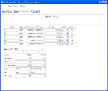
Fig. 10-2 Setting graph data
Users are able to change the labels, the scaling factors, and the color of the lines. Checking the checkbox of “not draw” omits its time evolution from the graph. The button [Re-calc] recalculates the scaling factors and the regions for the X/Y-axises. The table on the lower screen is set for the X/Y-axises. X indicates time, and Y the concentrations of variables. Clicking the [Draw graph] button (Fig. 10-2) displays the results of time-evolution data, as shown in Fig. 10-3.
.
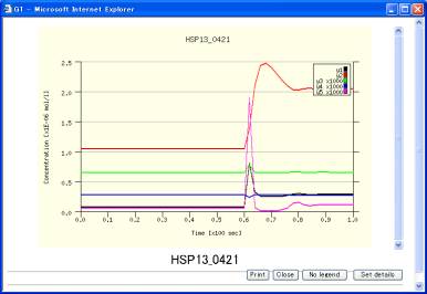
Fig. 10-3 Graph display
The [No legend] button omits the legends. The [Set details] button is able to change the color of the graph and other graph expressions. Clicking the [Set details] button displays the window (Fig.10-4). Users can change the style of the graph by inputting the value in the boxes. The values of the graph size and the location of the legends are determined by using pixel units. The location of the legend is determined by the coordinate of the left and upper legend.
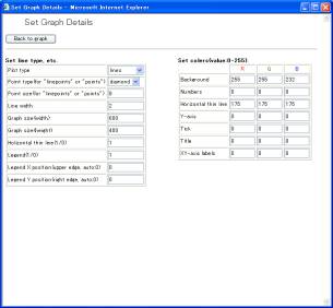
Fig. 10-4 Detailed setting for a graph