1. Login

Following the installation of the CADLIVE Simulator, open http://kurata01.bse.kyutech.ac.jp/TEST/Life/index.html　on a PC browser to display the screen(Fig. 1-1). Input the user name, subsequently his/her password to start up simulation.

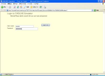
Fig. 1-1 Login screen

2. Startup simulator

Clicking the "Simulator" button on the left hand side (Fig. 2-1) changes the upper region of the screen, as shown in Fig.2-2

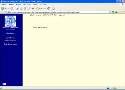
Fig. 2-1Startup menu

Fig. 2-2 Startup simulation

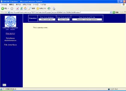
3. Upload of data for regulator-reaction equations

Clicking the [Regulator-reaction equations] button (Fig. 2-2) displays the new screen. Select the XML data file for the regulator-reaction equations (NFS_demo.xml) from users’ PC (Fig. 3-1). The data file should be described by using the CADLIVE Editors. Users are required to click the buttons within the screen of CADLIVE, not to carelessly click those of the browser.

Fig. 3-1 Upload of a regulator-reaction equation file from a PC

4. Selection of conversion methods

The table that indicates the selected regulator-reaction equations appears on the screen (Fig. 4-1). Users choose the conversion method with respect to gene-protein layer and metabolic layer.Select TPP_RAPID and MM, respectively.

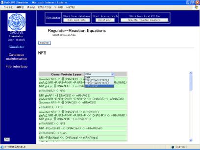
Fig. 4-1 Selection of conversion methods

Following the selection of the conversion method, clicking the [Confirm] button displays the confirmation screen (Fig. 4-2) that is similar to Fig. 4-1.

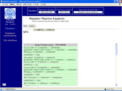
Fig. 4-2 Confirmation screen for the regulator-reaction equations

5. Editing Mathematical Model (DAEs)

Clicking the [Submit] button on the confirmation screen (Fig. 4-2) parses the regulator-reaction equations, converting them into the mathematical model according to the selected conversion method. The resultant mathematical model is displayed as shown in Fig. 5-1.

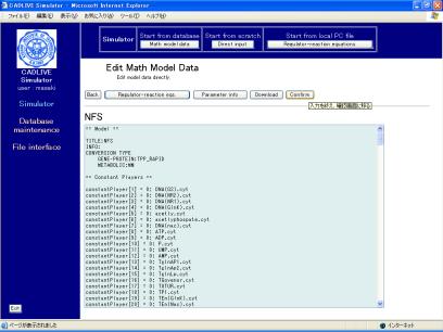
Fig. 5-1 Mathematical model that is obtained from regulator-reaction equations

This screen mainly has seven parts: the header, the definition of constant players, the definition of variables, the definition of the employed parameter labels, the definition of kinetic parameters, the definition of intermediate mathematical expressions, the definition of algebraic equations, and the definition of differential equations.

Clicking the [Regulator-reaction eqs.] button displays another window that shows regulator-reaction equations. Clicking the [Parameter info.] button shows the parameter information. The [Download] button enables users to download various data files to their local PC.

Clicking the [Confirm] button displays the confirmation screen (Fig. 5-2) that is similar to Fig. 5-1. If there is no problem, click the [Submit] button.

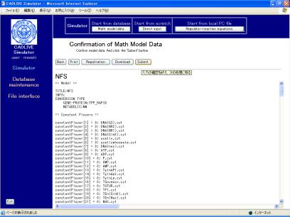
Fig. 5-2 Confirmation screen for a mathematical model

6. Selecting analysis types

Clicking the [Submit] button on the confirmation screen displays the screen (Fig. 6-1), where users select the method for numerical simulation. Select “Steady-state” as analysis type.

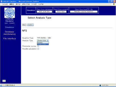
Fig. 6-1Selection of analysis type

As "Analsys type", users can choose either “Dynamic” or “Steady-state”. “ Dynamic” simulates the time evolution of the concentrations by calculating DAEs, and “Steady-state” calculates the concentrations at steady state by solving algebraic equations. The checkbox of "Parameter survey" determines if the simulator surveys the parameter space. Checking the checkbox of "Parallel calculation" carries out parallel calculation that employs the Message Passing Interface (MPI). Notice that the checkbox of "Parallel calculation" cannot be selected prior to checking the parameter survey.

7 Input for control data

Clicking the [Submit] button on the screen for selecting analytical type displays the screen for input of the control data (Fig. 7-1). Here, input the data, as provided by the following table.

Table Control parameters

Set values for Newton-Raphson Method.
Maximum trial times	20
Tolerance for convergence of functions	1e-16
Tolerance for convergence of variables	1e-16
Ratio of changing parameters	1.1
Change width for calc. sensitivity (STD)	0.001
Other
G-value	1.0
Y default value	0.01

Change width for calc. sensitivity (STD) means the ratio of the change in the kinetic parameters to their values, which is used to calculate the sensitivity of the dependent variables (concentrations) to the change in the kinetic parameters.

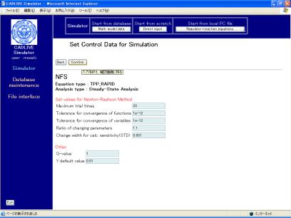
Fig. 7-1 Set control data for simulation

Following data input, clicking the [Confirm] button shows the confirmation screen (Fig. 7-2).

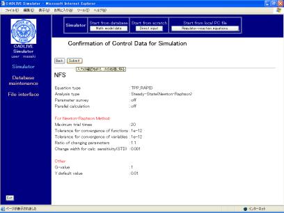
Fig. 7-2 Confirmation screen

8. Input of parameters

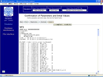
Following confirming the control data for simulation, clicking the [Submit] button on the screen (Fig. 7-2) displays the new screen (Fig. 8-1), where users input the kinetic parameters and initial values.

Fig. 8-1 Setting parameters and initial values

In this example, we presented the parameters and initial values that well simulated the ammonia assimilation system. Click the [Upload & merge File] button to display the screen (Fig. 8-2).

Fig. 8-2 Uploading a parameter file from the local PC

The parameter file that has been made (TPP_Param_NFS.txt) should be input in the box of "FileName". Check the box of "Update all" and click the [Submit] button. The parameters and initial values are automatically input into the mathematical model, as shown in Fig. 8-3

Fig. 8-3 Uploaded parameters and initial values

Following clicking the [Confirm] button, clicking the [Submit] button (Fig. 8-4) starts calculation.

Fig. 8-4 Startup calculation

9. Result indication

The results of the steady state concentrations and the sensitivity are shown in Fig. 9-1. The button of [Save for input] stores the resultant data as the initial values for the subsequent simulation (Fig. 9-1), which will be obtained by the [Initial val.] button. The steady state concentrations can be saved for the subsequent analysis (S-system analysis, simulation of DAEs). This [Initial val.] button will be not displayed when parameter survey has been carried out.

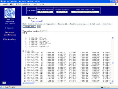
Fig. 9-1 Results

The screens for indicating the results (Fig. 9-1) have the [Registration] button. Clicking the [Registration] button shows the “Registration to the DB” screen (Fig. 9-2) that has also the button of [Registration]. Clicking it saves the steady state concentrations, and a series of sensitivity as a mathematical model in the database.

Fig. 9-2 Registration of Data in Database

The screen for results (Fig. 9-2) has the [Download] button. Clicking it displays the download screen (Fig. 9-3). The clicked files are downloaded to a local PC.

Fig. 9-3 Download