Grid Layout
CADLIVE TOP Grid Layout Last update August 23, 2010- What is a grid layout
- How to make grid layouts of graphs
- How to make grid layouts for CADLIVE networks
- About Graph representation of biochemical networks
- Downloads
- Some grid layout examples (Supplementary Materials to our grid layout Bioinformatics paper)
- Contacts
What is a grid layout
A grid layout is a special kind of graph layout, where all graph nodes are placed on a 2-dimensional squared grid. We developed an algorithm to compute grid layouts for graphs. In our approach, a graph is modeled as a system of interacting particles (nodes) on a given grid. The nodes interact according to a cost function which is designed based on the topological structure of the network. In such a system, closely related nodes attract each other, and remotely related nodes repulse each other.
We express our network layout method as an optimization algorithm which aims at finding optimized solutions of a certain objective cost that is a function of layouts of the input network. The network is modeled as a system of interacting particles which are placed on a 2-dimensional squared grid. The network is confined within an area L. The particles (nodes) interact according to a predefined energy function based on the network topological structure. A configuration of the particles represents a layout of the network, in which all edges are simple straight lines. The energy of a configuration is the cost score of the corresponding layout. A stable configuration has low energy; equivalently, an acceptable layout has a low cost score.
Back to topHow to make grid layouts for graphs
Grid layouts are calculated by the Windows program GLayout.exe, which accepts node list file as input. A graph is defined by a node list file, which consists of a list of node pairs that represent the edges of the graph. A node list file is a simple plain text file as follows:
nodeA nodeB
nodeB nodeC
nodeC nodeA
nodeC nodeD
Suppose that a graph is given by the node list file example.nls. (The node list file must end with the extension ".nls".) The following Windows shell command invokes GLayout.exe to compute a grid layout for the example:
GLayout example
The output is written to file example.nxy, which contains the node coordinates of the input graph. A node coordinates must have the extension .nxy, the format of which is as follows:
nodeA 1 3
nodeB 2 2
nodeC 3 2
nodeD 1 2
In the above file, the coordinates of nodeA, nodeB, nodeC, and nodeD are (1,3), (2,2), (3,2), and (1,2), respectively.
Note:
How to make grid layouts for CADLIVE networks
CADLIVE networks are stored in an XML format, which complies with the sanac specification. GLayout cannot read data directly from CADLIVE XML files; it reads network data only in node list format. Its output is a file of nodes and corresponding coordinates. To read CADLIVE network data and visualize layout in CADLIVE software, pCADLIVE should be used. pCADLIVE is designed to communicate between GLayout and CADLIVE XML data files. The usage of pCADLIVE.exe is:
pCADLIVE < inputfile >
The input file must be either a CADLIVE XML file (with extension .xml) or a node coordinates file (with extension .nxy).The whole process of making a grid layout of a CADLIVE network consists of 3 steps:
The following example illustrates how to make a grid layout for the CADLIVE network given by cell_cycle.xml. Make sure that sanac.dtd is in the same folder.
sanac.dtd is in the same folder.
pCADLIVE cell_cycle.xml
GLayout cell_cycle
pCADLIVE cell_cycle.nxy
The first command reads the cell_cycle network in the sanac format and outputs a node list file named cell_cycle.nls. The second command reads this node list file, and computes the grid layout. The output is a node coordinates file named cell_cycle.nxy. The last command reads node coordinates from cell_cycle.nxy. According to the coordinates, all layout information needed by CADLIVE is calculated and then written to file new_cell_cycle.xml in sanac format. The network stored in file new_cell_cycle.xml is the same as that in cell_cycle.xml except the network layout.
When making grid layouts of CADLIVE networks, some conversion is needed. Because of the existence modifiers, a general CADLIVE network cannot be fully described by a node list file. We use this convention: If a modifier acts on a reaction arrow, two virtual edges are set to connect the modifier and the both end nodes of the arrow. The virtual edges play roles only in making grid layouts; they disappear when the networks are written back to the XML format which is used by CADLIVE.
About Graph representation of biochemical networks
In order to visualize gene regulatory and signal transduction pathways, we defined the notation of regulator-reaction equations and presented their graphical representation. A regulator-reaction equation is defined by
Regulator (Modifier) -0 Reactants -> Products
which clearly shows the relationship between regulators and their regulated reactions. The Systems Biology Markup Language (SBML) level 2 supports this formula. The symbols indicate an enzyme (-0), an activator (->>), or an inhibitor (-II). Reversible and irreversible reactions are described by the arrows (<->) and (->), respectively.
In a graph representation, a reaction is represented by a set of edges between the reactants, products, and regulators. When a regulator acts on a reaction represented by a single edge, a node connects to an edge instead of another node. Such "edges" are beyond the scope of usual graphs. This is not fully described by a graph representation without any modifications. In this layout system, when a regulator acts on a reaction arrow, two virtual edges are set to connect the regulator to the both end nodes of the arrow. The virtual edges are employed only in making grid layouts; they are omitted when the networks are visualized.
Some grid layout examples
|
This is also the Supplementary Materials for our paper Weijiang Li and Hiroyuki Kurata A grid layout algorithm for automatic drawing of biochemical networks Bioinformatics, 21(9):2036-2042, 2005. |
|---|
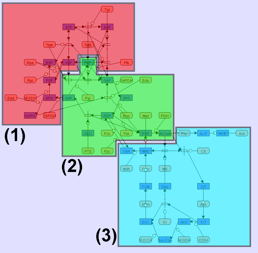
All examples here are visualized by CADLIVE. In the figures, the round rectangles are proteins, the rectangles metabolites, the parallelograms mRNAs, and ovals events. The solid black circles are complexes or modified molecules. The arrows indicate various reactions (binding, modification, conversion, transcription, translation, and transportation) or regulations (by an enzyme, activator, or inhibitor). Functional modules are marked by color blocks. In the figures, we used the abbreviated names of metabolites and enzymes to avoid drawing difficulties caused by some very long names.
Example 1. The yeast cell cycle regulatory network
Example 1a. The yeast cell cycle regulatory network generated by GraphViz
Downloads
Executable programs pCADLIVE.exe and GLayout.exe were built and tested under Windows XP. Microsoft .NET Framework 1.0 or above is needed to run the programs. If you do not have .NET framework, please install the .NET Framework Redistributable which is freely available from Microsoft download site.
Here we provide two sample CADLIVE networks, the yeast cell cycle (cell_cycle.xml) and the heat shock response network of E. coli (hsr_demo.xml). The original layouts of the two networks were made manually. Of course, GLayout has no relation to these layouts. Please note that the attached file sanac.dtd should be provided together with the .xml files in the same folder. sanac.dtd is the Document Type Definitions of CADLIVE XML data files.
The grid layout programs and the sample biochemical networks can be downloaded here. To visualize the layouts, you also need to download CADLIVE 2.75, which is free, too.
In CADLIVE, you can visualize a network (stored in an .xml file) by clicking the following menu items:
File -> Import -> Import a new network -> OK
and then choose the .xml file that you are interested in.